Matrix Representations of Modular Robots

Incidence Matricies

It is common to represent teams of modular robots as graphs. In this representation, a vertex is a single module and edge represents a connection between modules. A commonly used matrix representation for a graph is the incidence matrix. The incidence matrix, $M$, is an $n \times m$ matrix where the $ijth$ entry is a binary entry expressing if edge $m$ is connected to vertex $i$ or not. Each column, $j$, of $M$ represents an edge. The rows in an individual column represent the vertices that the edge is connecting. Given an example modular robot with its accompanying graph:

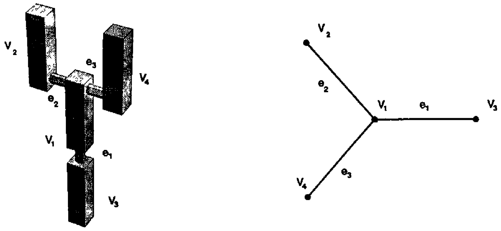
The incidence matrix for this modular robot is expressed as

$$M = \begin{bmatrix}1 & 1 & 1 \\ 0 & 1 & 0 \\ 1 & 0 & 0 \\ 0 & 0 & 1 \end{bmatrix}$$

When dealing with modular robots, it is not enough to simply know which modules are connected to which other modules. Sometimes a robot team will have multiple different types of modules as well as different ways to connect those modules. It is for this case that Chen and Burdick propose the extended incidence matrix, which augments the incidence matrix by adding one additional column and row [1].

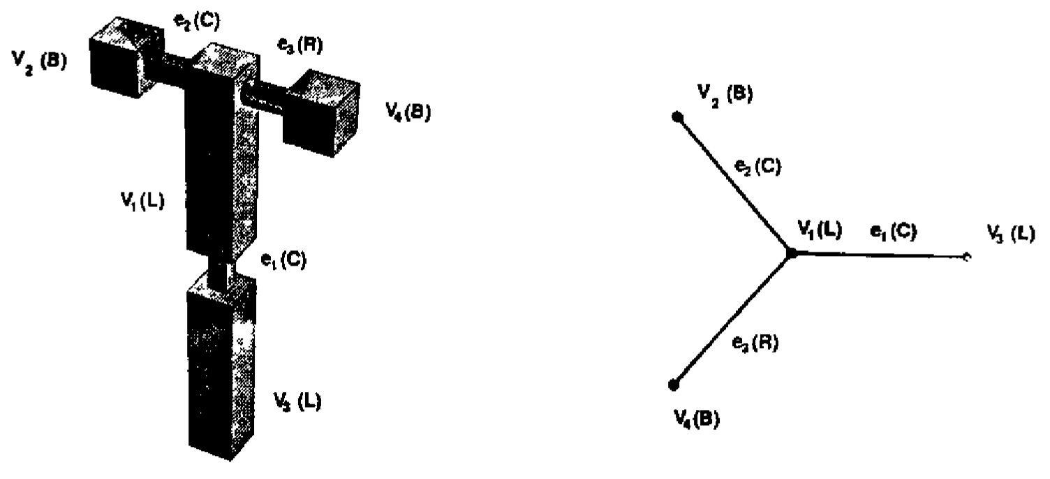
For the above nonhomogenous sample modular robot, the extended incidence matrix is denoted as:

$$M = \begin{bmatrix}1 & 1 & 1 & L \\ 0 & 1 & 0 & B \\ 1 & 0 & 0 & L \\ 0 & 0 & 1 & B \\ C & C & R & 0 \end{bmatrix}$$

Here, the end of each row denotes the type of module that the vertex represents; in this case $L$ or $B$. The bottom of each column represents the type of connection between the modules. This representation allows for a much more rich description of the modular robotic team beyond homogenous robots.

Assembly Incidence Matrices

Oftentimes, modules have a fixed number of connection ports. Knowing which connection ports are occupied may be important for finding valid reconfiguration paths through the configuration space. Chen and Burdick tackle this problem by introducing the assembly incidence matrix. This matrix is the same as the incidence matrix except instead of using $1$ to denote that there exists a connection and $0$ to denote that there is not a connection, the assembly incidence matrix uses a port number to denote that there is a connection at a particular port number. The nonhomogeneous modular robot example from before has an assembly incidence matrix of:

$$M = \begin{bmatrix}10 & 5 & 1 \\ 0 & 2 & 0 \\ 9 & 0 & 0 \\ 0 & 0 & 4 \end{bmatrix}$$

This is useful because if we know apriori the number of ports a robot has, we can know which ports are available for new connections. Similar to the incidence matrix, the assembly incidence matrix can be extended to represent the nonhomogenous module and connection information by augmenting it into the extended assembly incidence matrix, represented as:

$$M = \begin{bmatrix}10 & 5 & 1 & L \\ 0 & 2 & 0 & B \\ 9 & 0 & 0 & L \\ 0 & 0 & 4 & B \\ C & C & R & 0 \end{bmatrix}$$

These representations increase the amount of information that can be stored in matrix representations of modular robots. Later in the paper, the authors leverage this encoding as well as other algorithms to create an algorithm for enumeration of all non-isomorphic tree graphs. In the world of modular robotics, this is analogous to finding all possible chain type configurations.

Citations

[1] I.-M. Chen and J. W. Burdick, “Enumerating the nonisomorphic assembly configurations of modular robotic systems,” in Proceedings of 1993 IEEE/RSJ International Conference on Intelligent Robots and Systems (IROS ’93), Jul. 1993, pp. 1985–1992 vol.3. doi: 10.1109/IROS.1993.583905.