5-Bar Linkage Dynamic Simulation
The equations of motion were derived using an extension of the projection-based derivation of the equations of motion outline here. The basic method in the paper is as follows. Suppose that the equations of motion for a kinematically connected rigid mody can be written as.
$$M\ddot{X}+DM\dot{X}=G+G^{c}$$
Where $M$ is a diagonal matrix containing inertial values for each element the states, $X$ is the state vector, $D$ is a matrix containing centrifugal terms for each state element, $G$ is a vector containing the applied external forces, and $G^c$ is a vector containing the constraint forces due to kinematic constraints. Note that all values except for the constraint forces can be derived using only knowledge of the physical parameters of each rigid body.
Recognizing the relationship between the jacobian, $B$, and the applied independent coordinates vector, $q$
$$\dot{X} = B\dot{q}$$
We can then take the equations of motion and write them in terms of $q$
$$M(B\ddot{q} + \dot{B}\dot{q}) + DMB\dot{q} = G + G^c$$
The difficulty here is that the constraint forces are unknown. The method of projections solves this by multiplying the equations of motion by the transpose of the jacobian. This projects the constraint forces down to the zero vector. This is because, by definition, constraint forces cannot do work since they act orthogonally to the direction of motion. Therefore out equations of motion become
$$B^TMB\ddot{q} + (B^TM\dot{B}+B^TDMB)\dot{q} = B^TG$$
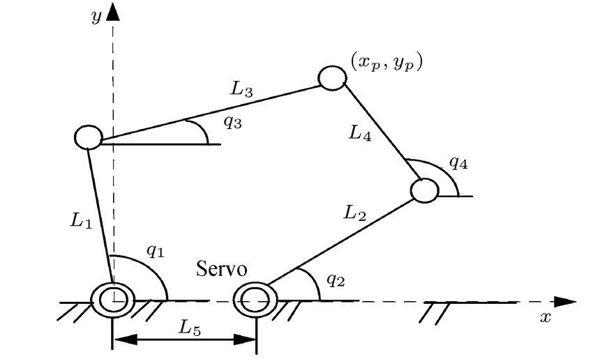
Now consider the five bar linkage:
As with any problem, we must first define the state vector:
$$X = \begin{bmatrix} X_1 \\ X_2 \\ X_3 \\ X_4 \end{bmatrix}$$
Where
$$X_i = \begin{bmatrix} x_i \\ y_i \\ \theta_i \end{bmatrix}$$
Here, $x_i$ and $y_i$ represent the x and y position of the center of mass with respect to the origin. $\theta_i$ represent the angle of the bar with respect to the horizontal (equivilant to $q_i$).
In order to apply method of projections to derive the dynamics of the five bar linkage, we must first recognize that while there are four angles, there are only two independent coordinates. This can be verified using Grübler’s formula for computation of degrees of freedom. Since $L_5$ is the ground link in this case, we know that $q_1$ and $q_2$ can be used to fully define $q_3$ and $q_4$. Put more simply
$$q_3(q_1, q_2), q_4(q_1, q_2)$$
And our independent coordinates vector becomes:
$$q = \begin{bmatrix} q_1 \\ q_2 \end{bmatrix}$$
Then we can define the following submatricies:
$$\dot{X}_1 = B_1\dot{q}$$ $$\dot{X}_2 = B_2\dot{q}$$ $$ \dot{X}_3 = B_3\dot{q}$$ $$ \dot{X}_4 = B_4\dot{q} $$
The full jacobian can be written as a 12 x 2 matrix as such:
$$B = \begin{bmatrix} B_1 \\ B_2 \\ B_3 \\ B_4 \end{bmatrix}$$
With the jacobian defined, we can then compute the equations of motion for the as described above:
$$B^TMB\ddot{q} + (B^TM\dot{B}+B^TDMB)\dot{q} = B^TG$$
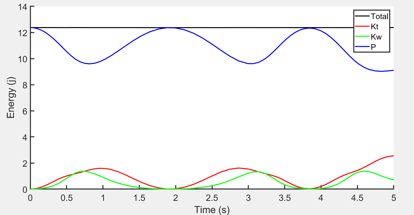
The actual implementation of this derivation was done symbolically in MATLAB. It required about 15 minutes running on 2019 Intel I7 processor. The derived equations of motion were stored in a separate file and simulations were conducted separatley. To validate the derivation, energy fluctuations were monitored under zero input, zero friction conditions. The figure below shoes that the total energy remained constant. This gives credence to the idea that the implementation was correct.